TidyTuesday 2020 Week 45

R setup

library(tidyverse)
library(tidytuesdayR)
library(gt)
library(rmarkdown)

library(dunnr)
extrafont::loadfonts(device = "win", quiet = TRUE)
theme_set(theme_td_grey())
set_geom_fonts()
set_palette()
ikea_colors <- c("#0051BA", "#FFDA1A")

Load the data

tt <- tt_load("2020-11-03")

The data this week comes from the Kaggle, and was the subject of a FiveThirtyEight article. See the Kaggle page for a data dictionary.

Data exploration

ikea <- tt$ikea %>% rename(row_number = `...1`)
glimpse(ikea)

Rows: 3,694
Columns: 14
$ row_number        <dbl> 0, 1, 2, 3, 4, 5, 6, 7, 8, 9, 10, 11, 12, 13, 14, 15…
$ item_id           <dbl> 90420332, 368814, 9333523, 80155205, 30180504, 10122…
$ name              <chr> "FREKVENS", "NORDVIKEN", "NORDVIKEN / NORDVIKEN", "S…
$ category          <chr> "Bar furniture", "Bar furniture", "Bar furniture", "…
$ price             <dbl> 265, 995, 2095, 69, 225, 345, 129, 195, 129, 2176, 1…
$ old_price         <chr> "No old price", "No old price", "No old price", "No …
$ sellable_online   <lgl> TRUE, FALSE, FALSE, TRUE, TRUE, TRUE, TRUE, TRUE, TR…
$ link              <chr> "https://www.ikea.com/sa/en/p/frekvens-bar-table-in-…
$ other_colors      <chr> "No", "No", "No", "Yes", "No", "No", "No", "No", "No…
$ short_description <chr> "        Bar table, in/outdoor,          51x51 cm", …
$ designer          <chr> "Nicholai Wiig Hansen", "Francis Cayouette", "Franci…
$ depth             <dbl> NA, NA, NA, 50, 60, 45, 44, 50, 44, NA, 44, 45, 47, …
$ height            <dbl> 99, 105, NA, 100, 43, 91, 95, NA, 95, NA, 103, 102, …
$ width             <dbl> 51, 80, NA, 60, 74, 40, 50, 50, 50, NA, 52, 40, 46, …

Are there duplicate names?

ikea %>%
  count(name, sort = T)

# A tibble: 607 × 2
   name        n
   <chr>   <int>
 1 BESTÅ     173
 2 PAX       111
 3 GRÖNLID    83
 4 BEKANT     74
 5 TROFAST    74
 6 IVAR       69
 7 VIMLE      63
 8 EKET       61
 9 PLATSA     57
10 LIDHULT    52
# … with 597 more rows
# ℹ Use `print(n = ...)` to see more rows

Yes, quite a bit. 400 out of 3694 items have multiple entries. Take a look at one example with two entries, the “TOBIAS”:

ikea %>%
  filter(name == "TOBIAS") %>%
  mutate(across(everything(), as.character)) %>%
  pivot_longer(cols = -row_number, names_to = "variable") %>%
  pivot_wider(names_from = row_number, values_from = value) %>%
  gt() %>%
  tab_spanner(label = "row number", columns = -variable)

variable	row number
	1167	1501
item_id	80349671	60334722
name	TOBIAS	TOBIAS
category	Chairs	Chairs
price	345	345
old_price	No old price	No old price
sellable_online	TRUE	TRUE
link	https://www.ikea.com/sa/en/p/tobias-chair-transparent-chrome-plated-80349671/	https://www.ikea.com/sa/en/p/tobias-chair-blue-chrome-plated-60334722/
other_colors	No	No
short_description	Chair	Chair
designer	Carl Öjerstam	Carl Öjerstam
depth	56	56
height	82	82
width	55	55

In the data, these are basically identical. Looking at the actual web page, I see that these are two different colors of the same item. Seems to me that it should have been a single entry with other_colors = “Yes”.

Likewise, the item_id variable is not unique – there are 2962 distinct values for 3694 items. It turns out this has to do with a single entry consisting of multiple items, for example this table and chairs:

ikea %>%
  filter(item_id == 49011766) %>%
  mutate(across(everything(), as.character)) %>%
  pivot_longer(cols = -row_number, names_to = "variable") %>%
  pivot_wider(names_from = row_number, values_from = value) %>%
  gt() %>%
  tab_spanner(label = "row number", columns = -variable)

variable	row number
	1121	2631
item_id	49011766	49011766
name	MELLTORP / ADDE	MELLTORP / ADDE
category	Chairs	Tables & desks
price	179	179
old_price	SR 205	SR 205
sellable_online	TRUE	TRUE
link	https://www.ikea.com/sa/en/p/melltorp-adde-table-and-2-chairs-white-s49011766/	https://www.ikea.com/sa/en/p/melltorp-adde-table-and-2-chairs-white-s49011766/
other_colors	No	No
short_description	Table and 2 chairs, 75 cm	Table and 2 chairs, 75 cm
designer	Lisa Norinder/Marcus Arvonen	Lisa Norinder/Marcus Arvonen
depth	NA	NA
height	72	72
width	75	75

Because this entry consists of chairs and a table, it falls under the “Chairs” and “Tables & desks” categories, despite being identical.

The category variable has the following distribution:

ikea %>%
  count(category, sort = T) %>%
  paged_table()

The price variable is the cost in Saudi Riyals at the time of data extraction:

ikea %>%
  ggplot(aes(x = price)) +
  geom_boxplot(aes(y = 0), outlier.shape = NA) +
  geom_jitter(aes(y = 1), alpha = 0.2) +
  scale_x_log10(breaks = c(1, 10, 100, 1000, 10000)) +
  dunnr::remove_axis("y")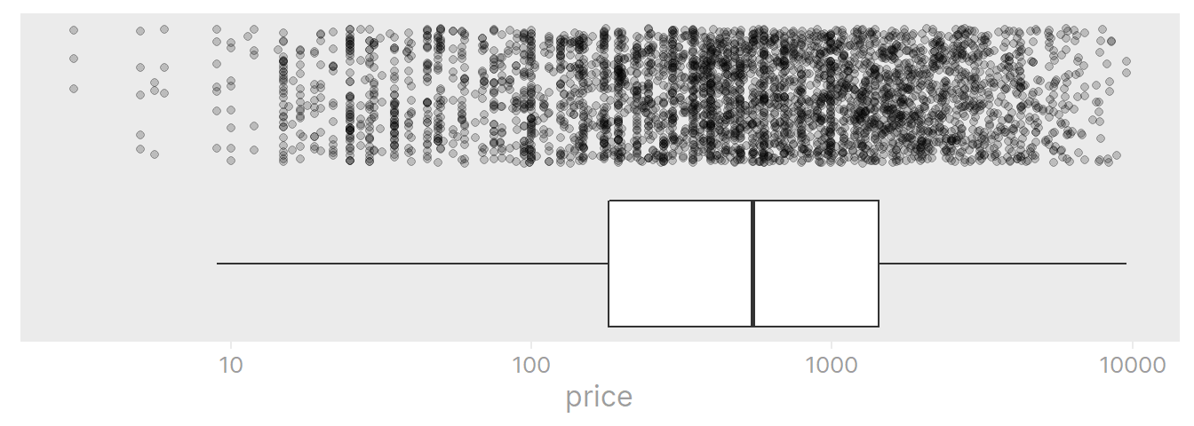

Out of curiosity, look at the top and bottom 3 items by price (and convert it to Canadian dollars for my own reference):

slice_max(ikea, price, n = 3) %>% mutate(price_group = "Most expensive") %>%
  bind_rows(
    slice_min(ikea, price, n = 3) %>% mutate(price_group = "Least expensive")
  ) %>%
  arrange(price) %>%
  transmute(
    price_group, name, category, short_description, price,
    # Exchange rate as of writing this
    price_cad = round(price * 0.34),
    # Put the URL into a clickable link
    link = map(link,
               ~gt::html(as.character(htmltools::a(href = .x, "Link")))),
  ) %>%
  group_by(price_group) %>%
  gt()

name	category	short_description	price	price_cad	link
Least expensive
GUBBARP	Bookcases & shelving units	Knob, 21 mm	3	1	Link
GUBBARP	Cabinets & cupboards	Knob, 21 mm	3	1	Link
GUBBARP	TV & media furniture	Knob, 21 mm	3	1	Link
Most expensive
GRÖNLID	Sofas & armchairs	U-shaped sofa, 6 seat	8900	3026	Link
LIDHULT	Beds	Corner sofa-bed, 6-seat	9585	3259	Link
LIDHULT	Sofas & armchairs	Corner sofa-bed, 6-seat	9585	3259	Link

The most expensive items are 6-seat sofas, and the least expensive are drawer knobs.

The old_price variable is, according to the data dictionary, the price before discount:

ikea %>%
  count(old_price, sort = T) %>%
  paged_table()

Most of the time, there is “No old price”, which I’ll replace with NA. Every other value is a price in Saudia Riyals, which I will convert to numeric. Before that, we need to consider a handful of items that are priced in packs:

ikea %>%
  filter(str_detect(old_price, "pack")) %>%
  select(name, category, price, old_price, link)

# A tibble: 10 × 5
   name      category                   price old_price     link                
   <chr>     <chr>                      <dbl> <chr>         <chr>               
 1 BRYNILEN  Beds                          30 SR 50/4 pack  https://www.ikea.co…
 2 BRENNÅSEN Beds                          30 SR 50/4 pack  https://www.ikea.co…
 3 BURFJORD  Beds                          40 SR 50/4 pack  https://www.ikea.co…
 4 BÅTSFJORD Beds                          30 SR 50/4 pack  https://www.ikea.co…
 5 BJORLI    Beds                          40 SR 50/4 pack  https://www.ikea.co…
 6 SKÅDIS    Bookcases & shelving units     6 SR 10/4 pack  https://www.ikea.co…
 7 SJÄLLAND  Outdoor furniture            356 SR 445/2 pack https://www.ikea.co…
 8 NORSBORG  Sofas & armchairs             80 SR 100/4 pack https://www.ikea.co…
 9 NORSBORG  Sofas & armchairs            140 SR 175/2 pack https://www.ikea.co…
10 NORSBORG  Sofas & armchairs             80 SR 100/4 pack https://www.ikea.co…

Looking at a few of the links for these items, and from the fact that the price is always less than old_price, both of the prices should be for the same number of items in a pack, so I shouldn’t need to adjust the prices by unit.

ikea <- ikea %>%
  mutate(
    old_price = readr::parse_number(old_price, na = "No old price"),
    # Also compute the percentage discount
    perc_discount = ifelse(is.na(old_price), 0.0,
                           (old_price - price) / old_price)
  )

Now compare price and old_price for the 654 items with both (I split up items into quartiles of price to separate the data a bit):

ikea %>%
  filter(!is.na(old_price)) %>%
  # For ease of visualization, separate the items by their price range
  mutate(
    price_range = cut(
      price,
      breaks = quantile(price, c(0, 0.25, 0.5, 0.75, 1.0)), include.lowest = T,
      labels = c("1st quartile", "2nd quartile", "3rd quartile", "4th quartile")
    )
  ) %>%
  select(row_number, price_range, price, old_price, perc_discount) %>%
  pivot_longer(cols = c(old_price, price)) %>%
  ggplot(aes(x = name, y = value)) +
  geom_point() +
  geom_line(aes(group = row_number, color = perc_discount), alpha = 0.4) +
  scale_y_log10("Price in SAR") +
  facet_wrap(~price_range, ncol = 2, scales = "free_y") +
  scale_color_gradient2(
    "Percent discount",
    low = td_colors$div5[1], mid = td_colors$div5[3], high = td_colors$div5[5],
    labels = scales::percent_format(1), midpoint = 0.25
  )

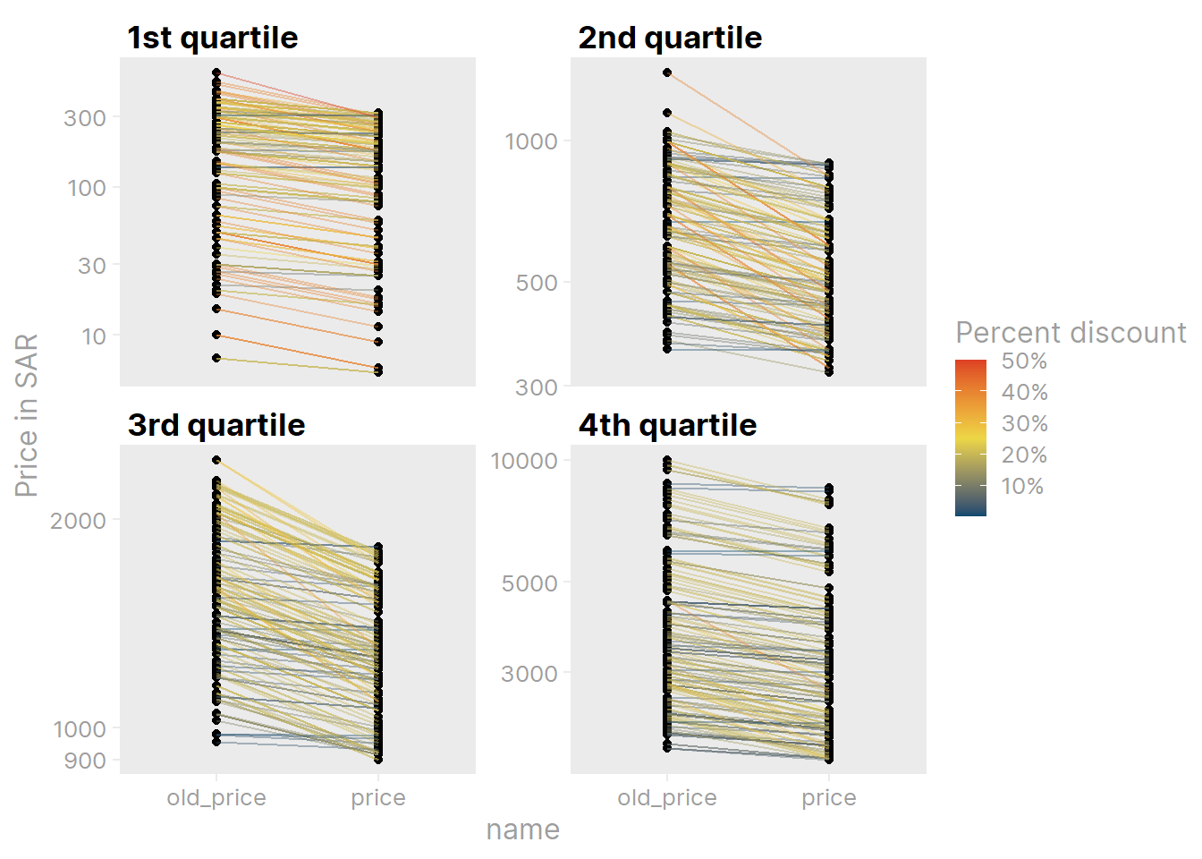
It looks like there may be a relationship between an item’s price and its discount, which we can look at directly:

ikea %>%
  filter(!is.na(old_price)) %>%
  ggplot(aes(x = old_price, y = perc_discount)) +
  geom_point(alpha = 0.5) +
  geom_smooth(method = "loess", formula = "y ~ x") +
  scale_x_log10() +
  scale_y_continuous(labels = scales::percent_format(1))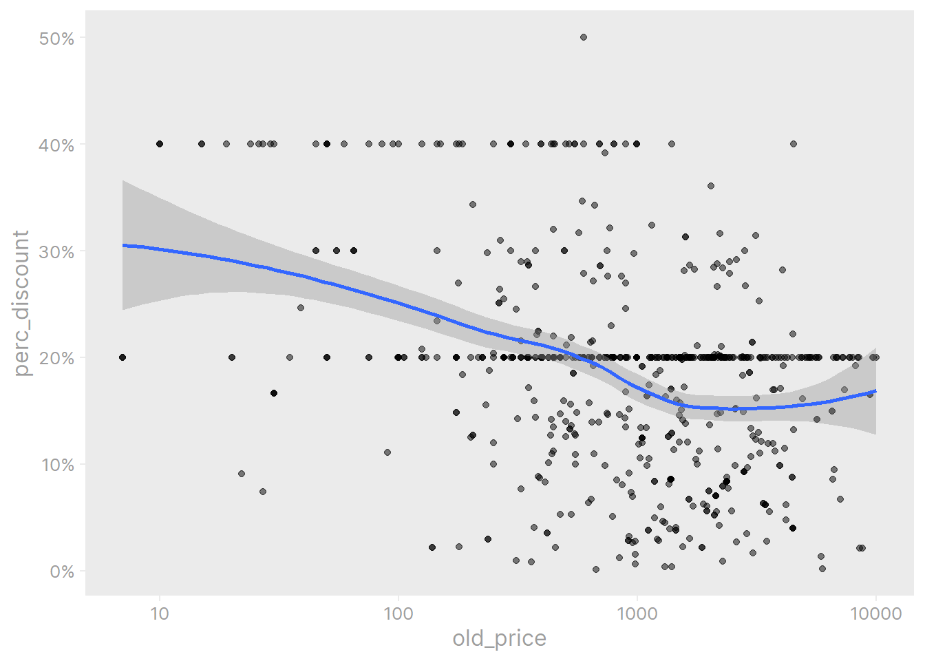

Yes, the more expensive items are less likely discounted by more than 20%. Cheaper items (old_price < 100) are most often discounted by 40%.

The sellable_online variable is logical:

ikea %>% count(sellable_online)

# A tibble: 2 × 2
  sellable_online     n
  <lgl>           <int>
1 FALSE              28
2 TRUE             3666

The 28 items which are not sellable online:

ikea %>%
  filter(!sellable_online) %>%
  select(name, category, price, short_description) %>%
  paged_table()

The other_colors variable is “Yes” or “No”, which I’ll convert to a logical:

ikea <- ikea %>% mutate(other_colors = other_colors == "Yes")
ikea %>% count(other_colors)

# A tibble: 2 × 2
  other_colors     n
  <lgl>        <int>
1 FALSE         2182
2 TRUE          1512

Is there any relationship between price and other_colors? Try a simple t-test:

t.test(price ~ other_colors, data = ikea)

    Welch Two Sample t-test

data:  price by other_colors
t = -4.9283, df = 2944.3, p-value = 8.754e-07
alternative hypothesis: true difference in means between group FALSE and group TRUE is not equal to 0
95 percent confidence interval:
 -324.0042 -139.5679
sample estimates:
mean in group FALSE  mean in group TRUE 
           983.3355           1215.1216 

Yes, items that do not come in other colors are less expensive on average.

ikea %>%
  ggplot(aes(y = other_colors, x = price)) +
  geom_jitter(alpha = 0.2) +
  scale_x_log10()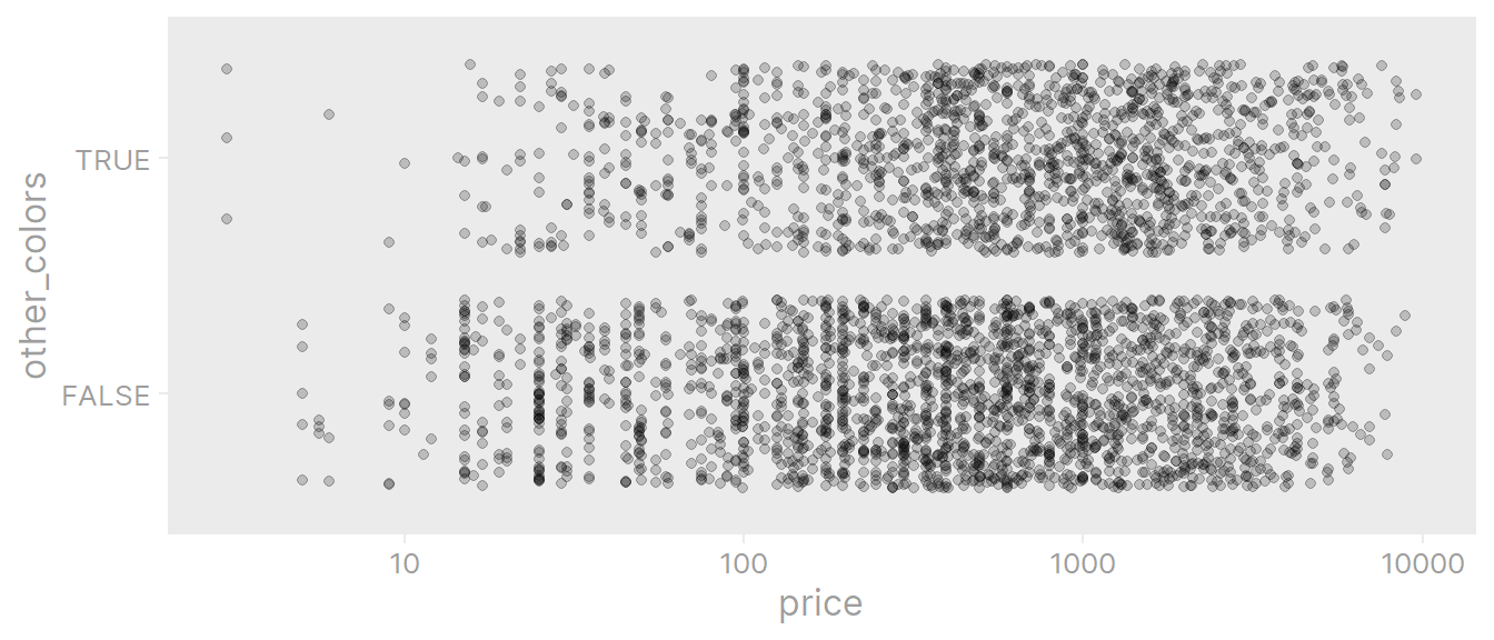

Doesn’t really pass the eye test though – the distributions are near identical. The magic of large sample sizes.

Short description

There are 1706 unique short_descriptions with the following counts:

# The short_description has a lot of white space issues, which we can
#  trim and squish
ikea <- ikea %>%
  mutate(
    short_description = short_description %>% str_trim() %>% str_squish()
  )

ikea %>%
  count(short_description, sort = T) %>%
  paged_table()

The first notable pattern is that the description often includes dimensions in centimeters, but it doesn’t seem to align with the dimension variables (heigth, width, depth). As an example, consider this item:

ikea %>%
  filter(row_number == 1156) %>%
  glimpse()

Rows: 1
Columns: 15
$ row_number        <dbl> 1156
$ item_id           <dbl> 99014376
$ name              <chr> "MELLTORP / ADDE"
$ category          <chr> "Chairs"
$ price             <dbl> 359
$ old_price         <dbl> NA
$ sellable_online   <lgl> TRUE
$ link              <chr> "https://www.ikea.com/sa/en/p/melltorp-adde-table-an…
$ other_colors      <lgl> FALSE
$ short_description <chr> "Table and 4 chairs, 125 cm"
$ designer          <chr> "Marcus Arvonen/Lisa Norinder"
$ depth             <dbl> NA
$ height            <dbl> 72
$ width             <dbl> 75
$ perc_discount     <dbl> 0

short_description has “125 cm”, but height = 72 and width = 75. Looking at the web page for the item, I can see that the 125 cm is the length of the table, which probably should have been imputed for the missing depth variable here.

I should be able to pull the dimensions out of the short_description with a regex:

# This regex looks for measurements in cm, mm and inches (") after a comma and
#  before the end of the string
# The complicated part is (,)(?!.*,) which is a negative lookahead that ensures
#  I only match the last comma of the text
dim_regex <- "(,)(?!.*,) (.*?) (cm|mm|\")$"
ikea <- ikea %>%
  mutate(
    short_description_dim = str_extract(short_description, dim_regex) %>%
      # Remove the comma
      str_remove(", "),
    # With the dimensions extracted, remove from the full short_description
    short_description = str_remove(short_description, dim_regex)
  )

Here is how that affected the example item:

ikea %>%
  filter(row_number == 1156) %>%
  select(short_description, short_description_dim)

# A tibble: 1 × 2
  short_description  short_description_dim
  <chr>              <chr>                
1 Table and 4 chairs 125 cm               

For the remaining text in short_description, we might be able to text mine some useful information to better categorize items. For instance, consider the category = “Chairs”:

ikea_chairs <- ikea %>% filter(category == "Chairs")
ikea_chairs %>%
  select(name, price, short_description) %>%
  paged_table()

Most of these are just single chairs or stools. But others are a table and multiple chairs:

ikea_chairs %>%
  filter(str_detect(short_description, "\\d+")) %>%
  select(price, short_description)

# A tibble: 156 × 2
   price short_description                 
   <dbl> <chr>                             
 1   179 Table and 2 chairs                
 2   359 Table and 4 chairs                
 3   549 Table and 4 chairs                
 4   495 Storage bench w towel rail/4 hooks
 5   589 Table and 2 chairs                
 6   285 Table and 4 chairs                
 7   145 Stepladder, 3 steps               
 8   289 Table and 2 chairs                
 9   579 Table and 4 chairs                
10   889 Table and 2 chairs                
# … with 146 more rows
# ℹ Use `print(n = ...)` to see more rows

I think a way to operationalize these descriptions is to extract the number of chairs/stools and indicate if there is a table:

chairs_regex <- "\\d (.*?)chair"
stools_regex <- "\\d (.*?)stool"
ikea <- ikea %>%
  mutate(
    # Count chairs
    chairs = str_extract(short_description, chairs_regex) %>%
      readr::parse_number(),
    chairs = ifelse(
      # If not multiple chairs
      is.na(chairs),
      # There is 0 or 1 chair
      as.numeric(str_detect(short_description,
                            regex("chair", ignore_case = TRUE))), chairs
    ),
    # Count stools
    stools = str_extract(short_description, stools_regex) %>%
      readr::parse_number(),
    stools = ifelse(
      # If not multiple stools
      is.na(stools),
      # There is 0 or 1 stools
      as.numeric(str_detect(short_description,
                            regex("stool", ignore_case = TRUE))), stools
    ),
    # Just look for 1 or 0 tables
    tables = as.integer(str_detect(short_description,
                                   regex("table", ignore_case = TRUE)))
  )
ikea %>%
  filter(chairs > 0 | stools > 0 | tables > 0) %>%
  count(short_description, chairs, stools, tables, sort = T)

# A tibble: 185 × 5
   short_description          chairs stools tables     n
   <chr>                       <dbl>  <dbl>  <int> <int>
 1 Table and 4 chairs              4      0      1   166
 2 Table                           0      0      1   132
 3 Table and 6 chairs              6      0      1    78
 4 Chair                           1      0      0    59
 5 Table and 2 chairs              2      0      1    34
 6 Armchair                        1      0      0    30
 7 Bar stool with backrest         0      1      0    25
 8 Coffee table                    0      0      1    25
 9 Table top                       0      0      1    22
10 Bar table and 2 bar stools      0      2      1    20
# … with 175 more rows
# ℹ Use `print(n = ...)` to see more rows

It’s not perfect feature engineering – the “Chair pad” item (16 occurrences) isn’t actually a chair, for instance – but these variables should be helpful in predicting prices.

ikea %>%
  filter(stools > 0 | chairs > 0) %>%
  # No items have both chairs and stools, so split them into groups
  mutate(chair_stool = ifelse(stools > 0, "stools", "chairs"),
         chair_stool_count = chairs + stools) %>%
  ggplot(aes(x = factor(chair_stool_count, levels = 1:8), y = price,
             color = factor(tables))) +
  geom_jitter(alpha = 0.5, height = 0, width = 0.2) +
  facet_wrap(~chair_stool) +
  dunnr::add_facet_borders() +
  labs(x = "chair/stool count", color = "tables") +
  theme(legend.position = c(0.9, 0.8)) +
  scale_y_log10() +
  scale_color_manual(values = ikea_colors) +
  dunnr::theme_td_grey()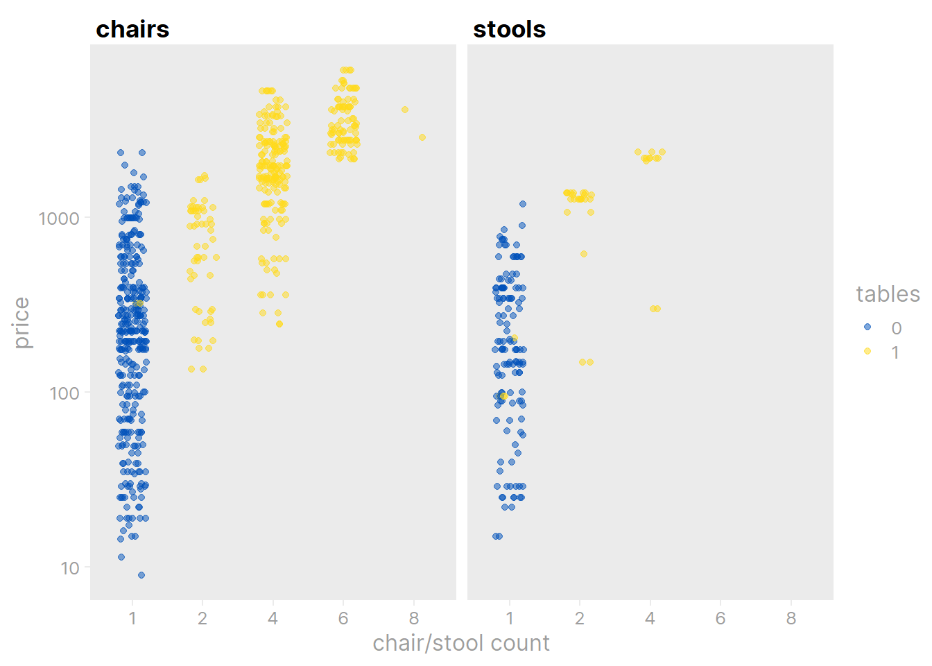

Our new variables are, unsurprisingly, very predictive of price. We can estimate the effects with a simple linear regression model:

lm(
  log(price) ~ chair_stool_count + tables,
  data = ikea %>%
    filter(stools > 0 | chairs > 0) %>%
    mutate(chair_stool_count = chairs + stools)
) %>%
  gtsummary::tbl_regression()

Characteristic	Beta	95% CI1	p-value
chair_stool_count	0.41	0.34, 0.48	<0.001
tables	0.91	0.66, 1.2	<0.001
1 CI = Confidence Interval

Both the number of stools/chairs and the presence of a table are highly significant predictors of item price.

We can also extract some useful variables for sofas. Here are the short_descriptions under the category “Sofas & armchairs”:

ikea_sofas <- ikea %>%
  filter(category == "Sofas & armchairs")
ikea_sofas %>%
  count(short_description, sort = T) %>%
  paged_table()

The number of seats can be extracted with some more regex:

# Find the sofas and sectionals
sofa_sectional_idx <-
  str_detect(ikea_sofas$short_description,
             regex("sofa|section", ignore_case = TRUE)) &
  # Exclude sofa covers and legs
  str_detect(ikea_sofas$short_description,
             regex("cover|leg", ignore_case = TRUE), negate = TRUE)

ikea_sofas <- ikea_sofas %>%
  mutate(
    sofa_seats = ifelse(
      sofa_sectional_idx,
      # Extract words or numbers before "-seat" or " seat"
      str_extract(short_description,
                  "(\\w+|\\d)(-| )seat"),
      NA_character_
    ),
    # If the description doesn't say the number of seats, then assume one seat
    sofa_seats = ifelse(
      sofa_sectional_idx & is.na(sofa_seats), "1-seat", sofa_seats
    )
  )

ikea_sofas %>%
  count(sofa_seats, short_description, sort = T) %>%
  filter(!is.na(sofa_seats))

# A tibble: 47 × 3
   sofa_seats short_description         n
   <chr>      <chr>                 <int>
 1 3-seat     3-seat sofa              30
 2 2-seat     2-seat sofa              18
 3 4-seat     4-seat sofa              16
 4 3-seat     3-seat sofa-bed          12
 5 4-seat     Corner sofa, 4-seat      12
 6 5-seat     Corner sofa, 5-seat      12
 7 1-seat     Corner section            7
 8 3-seat     3-seat section            7
 9 1-seat     Chaise longue section     6
10 2-seat     2-seat section            6
# … with 37 more rows
# ℹ Use `print(n = ...)` to see more rows

Now to convert this to a numeric variable, replace word representations (“two”, “three”) and use the readr::parse_number() function:

ikea_sofas <- ikea_sofas %>%
  mutate(
    sofa_seats = sofa_seats %>%
      tolower() %>%
      str_replace("two", "2")  %>%
      str_replace("three", "3") %>%
      readr::parse_number() %>%
      replace_na(0)
  )

And use logicals to indicate sofa beds and sectionals/modulars:

ikea_sofas <- ikea_sofas %>%
  mutate(
    sofa_bed = sofa_sectional_idx &
      str_detect(short_description, regex("sofa( |-)bed", ignore_case = T)),
    sofa_sectional = sofa_sectional_idx &
      str_detect(short_description, regex("modular|section", ignore_case = T))
  )

Plot the prices to see if there is an obvious relationship with these new variables:

ikea_sofas <- ikea_sofas %>%
  mutate(
    sofa_type = case_when(
      sofa_bed & sofa_sectional ~ "Bed + sectional",
      sofa_bed ~ "Bed",
      sofa_sectional ~ "Sectional",
      sofa_seats > 0 ~ "Normal",
      TRUE ~ "Not a sofa"
    )
  )
ikea_sofas %>%
  filter(sofa_type != "Not a sofa") %>%
  ggplot(aes(x = sofa_seats, y = log(price))) +
  geom_jitter(color = ikea_colors[1], height = 0, width = 0.11) +
  geom_smooth(color = ikea_colors[2], method = "lm", formula = "y ~ x") +
  facet_wrap(~sofa_type, ncol = 2) +
  theme_td_grey(gridlines = "xy")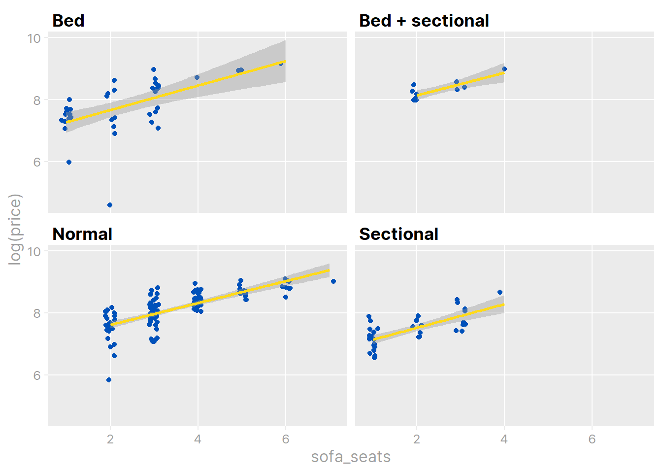

lm(
  log(price) ~ sofa_seats * sofa_type,
  data = ikea_sofas %>% filter(sofa_type != "Not a sofa") 
) %>%
  gtsummary::tbl_regression()

Characteristic	Beta	95% CI1	p-value
sofa_seats	0.39	0.29, 0.50	<0.001
sofa_type
Bed	—	—
Bed + sectional	0.53	-0.61, 1.7	0.4
Normal	0.03	-0.37, 0.42	0.9
Sectional	-0.12	-0.56, 0.32	0.6
sofa_seats * sofa_type
sofa_seats * Bed + sectional	-0.03	-0.46, 0.41	>0.9
sofa_seats * Normal	-0.04	-0.17, 0.09	0.5
sofa_seats * Sectional	-0.01	-0.21, 0.18	>0.9
1 CI = Confidence Interval

The sofa_type variable makes little difference, but the sofa_seats variable is definitely an important predictor of price in this subset of the data. Incorporate these variables into the larger data set:

Repeated code

# Find the sofas and sectionals
sofa_sectional_idx <-
  ikea$category == "Sofas & armchairs" &
  str_detect(ikea$short_description,
             regex("sofa|section", ignore_case = TRUE)) &
  # Exclude sofa covers and legs
  str_detect(ikea$short_description,
             regex("cover|leg", ignore_case = TRUE), negate = TRUE)

ikea <- ikea %>%
  mutate(
    sofa_seats = ifelse(
      sofa_sectional_idx,
      # Extract words or numbers before "-seat" or " seat"
      str_extract(short_description,
                  "(\\w+|\\d)(-| )seat"),
      NA_character_
    ),
    # If the description doesn't say the number of seats, then assume one seat
    sofa_seats = ifelse(
      sofa_sectional_idx & is.na(sofa_seats), "1-seat", sofa_seats
    ),
    sofa_seats = sofa_seats %>%
      tolower() %>%
      str_replace("two", "2")  %>%
      str_replace("three", "3") %>%
      readr::parse_number() %>%
      replace_na(0),
    sofa_bed = sofa_sectional_idx &
      str_detect(short_description, regex("sofa( |-)bed", ignore_case = T)),
    sofa_sectional = sofa_sectional_idx &
      str_detect(short_description, regex("modular|section", ignore_case = T)),
    sofa_type = case_when(
      sofa_bed & sofa_sectional ~ "Bed + sectional",
      sofa_bed ~ "Bed",
      sofa_sectional ~ "Sectional",
      sofa_seats > 0 ~ "Normal",
      TRUE ~ "Not a sofa"
    )
  )

Designer

Check out the designer variable:

ikea %>%
  count(designer, sort = TRUE) %>%
  paged_table()

There are a lot of unique designers unsurprisingly. One odd thing I noticed is that some of the designer values are not designer names, but rather additional descriptions of the items. Check the 3 longest designer values, for example:

ikea %>%
  slice_max(nchar(designer), n = 3, with_ties = FALSE) %>%
  select(name, short_description, designer, link) %>%
  paged_table()

Looking at the actual webpages for these items, it is clear that the designer variable was just incorrectly scraped from the website in these cases. Here is the distribution of string length:

ikea %>%
  ggplot(aes(x = nchar(designer), y = 0)) +
  geom_jitter(alpha = 0.1) +
  labs() +
  scale_x_log10(limits = c(1, 2e3)) +
  dunnr::remove_axis("y")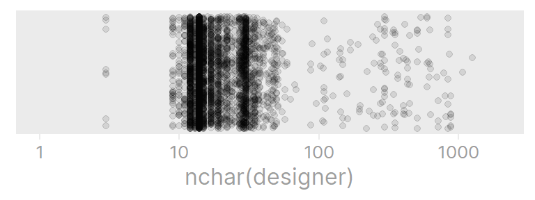

I’m sure there is some valuable information in these descriptions, but it would take a long time to extract that information. Instead I’ll use the fact that those designer values seem to begin with an “article number” like 104.114.40:

ikea %>%
  mutate(
    article_number = str_detect(designer, regex("^\\d+"))
  ) %>%
  ggplot(aes(x = nchar(designer), y = article_number, color = article_number)) +
  geom_jitter(alpha = 0.5, position = position_jitter(seed = 1), shape = 21,
              fill = "white") +
  scale_x_log10() +
  theme(legend.position = "none") +
  #geom_label(
  ggrepel::geom_text_repel(
    data = . %>% filter(article_number, nchar(designer) < 50),
    aes(label = designer),
    position = position_jitter(seed = 1), size = 3
  ) +
  scale_color_manual(values = rev(ikea_colors))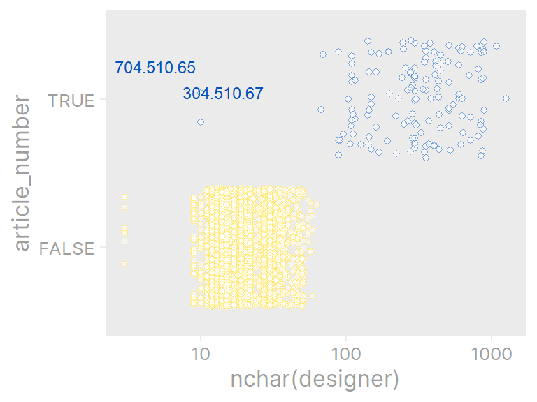

There were a couple cases of designer having the article number, but not being a long piece of text. These are the labelled points in the plot above (704.510.65 and 304.510.67). I’ll mark all of these designer values with article numbers as NA. Also of interest to me: does the price differ significantly when the designer is IKEA vs an individual?

ikea <- ikea %>%
  mutate(
    designer_group = case_when(
      str_detect(designer, regex("^\\d+")) ~ NA_character_,
      designer == "IKEA of Sweden" ~ "IKEA",
      str_detect(designer, "IKEA of Sweden") ~ "IKEA + individual(s)",
      str_detect(designer, "IKEA") ~ "oops",
      TRUE ~ "Individual(s)"
    ) %>%
      factor()
  )
ikea %>%
  filter(!is.na(designer_group)) %>%
  ggplot(aes(y = designer_group, x = price)) +
  geom_boxplot(outlier.shape = NA, width = 0.2) +
  geom_jitter(alpha = 0.1) +
  scale_x_log10()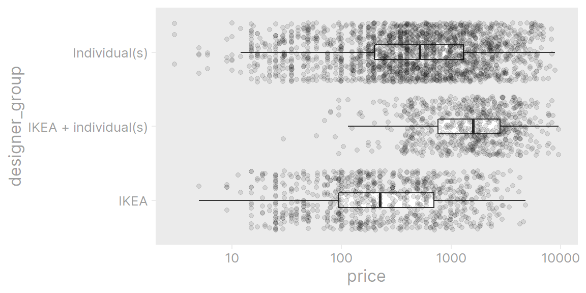

In general, items designed by IKEA alone are cheaper than items designed by one or more individuals, and items designed in collaboration with IKEA are the most expensive.

Size

The depth, height and width variables are all in centimeters. Summarize the values:

ikea %>%
  select(row_number, depth, height, width) %>%
  pivot_longer(cols = -row_number, names_to = "dimension") %>%
  group_by(dimension) %>%
  summarise(
    p_missing = mean(is.na(value)) %>% scales::percent(),
    median = median(value, na.rm = TRUE),
    min = min(value, na.rm = TRUE), max = max(value, na.rm = TRUE),
    .groups = "drop"
  ) %>%
  gt()

dimension	p_missing	median	min	max
depth	40%	47	1	257
height	27%	83	1	700
width	16%	80	1	420

Quite a few items are missing measurements and some of them are certainly wrong. A height of 700cm seems… unlikely. Looking at the link (https://www.ikea.com/sa/en/p/hilver-leg-cone-shaped-bamboo-80278273/), I see that it is actually 700mm, so this was an error in the data scraping. Take a look at the distribution of these values:

ikea %>%
  select(row_number, depth, height, width) %>%
  pivot_longer(cols = -row_number, names_to = "dimension") %>%
  filter(!is.na(value)) %>%
  ggplot(aes(y = dimension, x = value)) +
  geom_jitter(alpha = 0.4, color = ikea_colors[1], width = 0)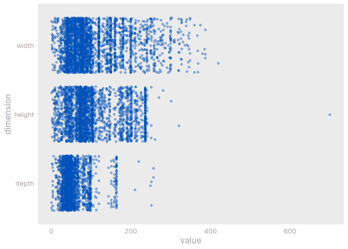

That is definitely the biggest outlier across all dimensions. There may be more incorrect values (e.g. maybe some of the smaller values are in meters), but I’ll just divide that one value of 700 by 10 (to convert it to centimeters) and be done with it for now.

ikea <- ikea %>%
  mutate(height = ifelse(height == 700, height / 10, height))

Now, for the values that we have, there should be an obvious relationship between price and size:

ikea %>%
  select(row_number, depth, height, width, price) %>%
  pivot_longer(cols = -c(row_number, price), names_to = "dimension") %>%
  filter(!is.na(value)) %>%
  ggplot(aes(x = value, y = log(price))) +
  geom_point(alpha = 0.5, color = ikea_colors[1]) +
  geom_smooth(method = "loess", formula = "y ~ x", color = ikea_colors[2]) +
  facet_wrap(~dimension, scales = "free_x") +
  theme_td_grey(gridlines = "xy")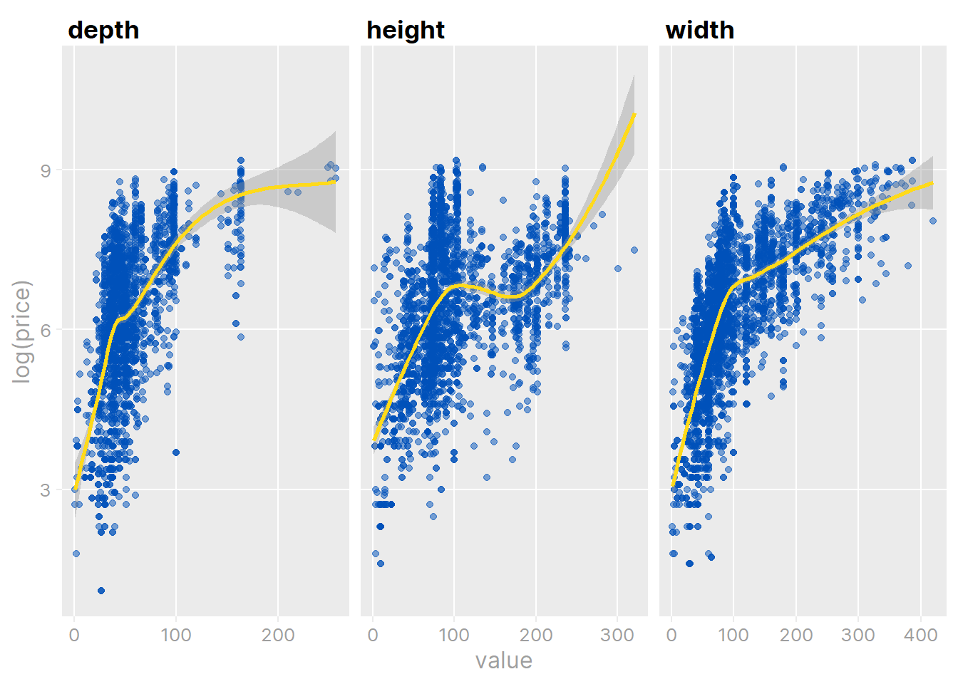

In all three cases, there is a positive non-linear relationship. The relationship between the three dimensions:

ikea %>%
  select(row_number, depth, height, width) %>%
  pivot_longer(cols = -row_number, names_to = "dimension") %>%
  filter(!is.na(value)) %>%
  mutate(dimension = factor(dimension)) %>%
  left_join(., ., by = "row_number") %>%
  # By converting the factor levels to an integer, the pairwise comparisons
  #  won't be duplicated
  filter(as.integer(dimension.x) > as.integer(dimension.y)) %>%
  mutate(dimension_comparison = str_c(dimension.x, " vs ", dimension.y)) %>%
  ggplot(aes(x = value.x, y = value.y)) +
  geom_point(alpha = 0.5, color = ikea_colors[1]) +
  geom_smooth(method = "loess", formula = "y ~ x", color = ikea_colors[2]) +
  facet_wrap(~dimension_comparison) +
  theme_td_grey(gridlines = "xy")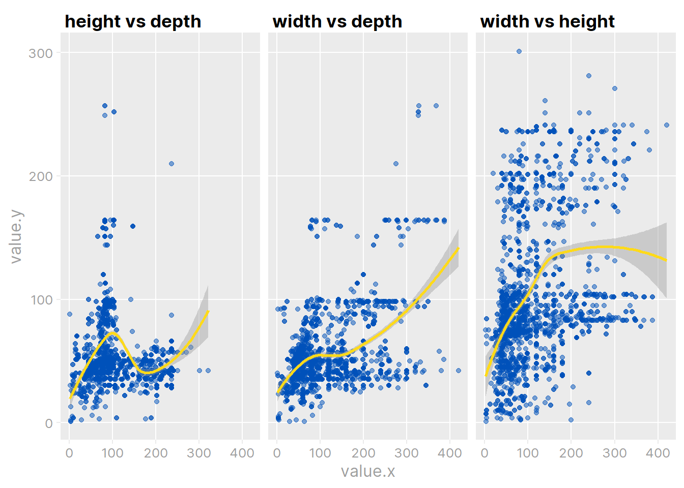

It is a very non-linear relationship, but generally monotonic. There is an interesting spike in depth around height \(\approx\) 100cm (in the left-most plot):

ikea %>%
  filter(depth > 150, height < 110, height > 90) %>%
  select(name, category, depth, height, width) %>%
  paged_table()

Mostly sofas and beds, which makes sense.

Model

I’ll attempt to predict item price with

• category, sellable_online, other_colors, depth, height, width from the original data, and
• perc_discount, chairs, stools, tables, sofa_seats, sofa_bed, sofa_sectional and designer_group from feature engineering.

Pre-processing

Convert the categorical variables to factors, and add log price as the outcome variable:

ikea <- ikea %>%
  mutate(across(where(is.character), factor),
         log_price = log10(price))

Load tidymodels and define the data split (75% training to 25% testing) and resampling:

library(tidymodels)
library(textrecipes) # For step_clean_levels()

set.seed(4)
ikea_split <- initial_split(ikea, prop = 3/4,
                            # Stratify by price
                            strata = log_price)
ikea_train <- training(ikea_split)
ikea_test <- testing(ikea_split)

# Use bootstrap resamples
ikea_bootstrap <- bootstraps(ikea_train, times = 25, strata = log_price)

Define the pre-processing recipe for the modelling pipeline:

ikea_rec <-
  recipe(
    log_price ~ category + sellable_online + other_colors +
      depth + height + width +
      perc_discount + chairs + stools + tables +
      sofa_seats + sofa_bed + sofa_sectional + designer_group,
    data = ikea_train
  ) %>%
  # The designer_group variable has missing values due to a scraping error,
  #  which we will simply impute with the most common value (the mode)
  step_impute_mode(designer_group) %>%
  # Too many categories for this model, so group low frequency levels
  step_other(category, threshold = 0.05) %>%
  # Impute dimension values with nearest neighbors (default k = 5)
  step_impute_knn(depth, height, width) %>%
  # Before turning into dummy variables, clean the factor levels
  textrecipes::step_clean_levels(all_nominal_predictors()) %>%
  # Turn our two nominal predictors (category and designer_group) to dummy vars
  step_dummy(all_nominal_predictors()) %>%
  # Remove variables with just a single value, if any
  step_zv(all_predictors())
ikea_rec

Recipe

Inputs:

      role #variables
   outcome          1
 predictor         14

Operations:

Mode imputation for designer_group
Collapsing factor levels for category
K-nearest neighbor imputation for depth, height, width
Cleaning factor levels for all_nominal_predictors()
Dummy variables from all_nominal_predictors()
Zero variance filter on all_predictors()

Before applying the recipe, we can explore the processing steps with the recipes::prep() and recipes::bake() functions applied to the training data:

ikea_baked <- bake(prep(ikea_rec), new_data = NULL)
ikea_baked %>% paged_table()

Check out the designer_group dummy variables:

ikea_baked %>%
  select(matches("designer_group")) %>%
  count(across(everything()))

# A tibble: 3 × 3
  designer_group_ikea_individual_s designer_group_individual_s     n
                             <dbl>                       <dbl> <int>
1                                0                           0   633
2                                0                           1  1637
3                                1                           0   500

Note that the 107 NA designer_group values were imputed with the most common value (the mode = “Individual(s)”):

ikea_train %>% count(designer_group)

# A tibble: 4 × 2
  designer_group           n
  <fct>                <int>
1 IKEA                   633
2 IKEA + individual(s)   500
3 Individual(s)         1530
4 <NA>                   107

The category variable was reduced to the following levels by collapsing low-frequency (<5%) levels into category_other:

ikea_baked %>%
  select(matches("category")) %>%
  count(across(everything())) %>%
  pivot_longer(cols = -n, names_to = "var") %>%
  filter(value == 1) %>%
  transmute(var, n, p = scales::percent(n / sum(n))) %>%
  arrange(desc(n)) %>%
  gt()

var	n	p
category_tables_desks	456	17.46%
category_bookcases_shelving_units	412	15.78%
category_other	357	13.67%
category_chairs	352	13.48%
category_sofas_armchairs	329	12.60%
category_cabinets_cupboards	214	8.20%
category_wardrobes	178	6.82%
category_outdoor_furniture	173	6.63%
category_tv_media_furniture	140	5.36%

The dimension variables height, depth and width were imputed by nearest neighbors (using the default \(k\) = 5). Summarise the values of each:

ikea_baked %>%
  select(height, depth, width) %>%
  mutate(idx = 1:n(), data = "ikea_baked") %>%
  bind_rows(
    ikea_train %>%
      select(height, depth, width) %>%
      mutate(idx = 1:n(), data = "ikea_train")
  ) %>%
  pivot_longer(cols = c(height, depth, width), names_to = "dim") %>%
  group_by(data, dim) %>%
  summarise(
    n = as.character(sum(!is.na(value))),
    p_missing = scales::percent(mean(is.na(value))),
    mean_val = as.character(round(mean(value, na.rm = TRUE), 1)),
    sd_val = as.character(round(sd(value, na.rm = TRUE), 1)),
    .groups = "drop"
  ) %>%
  pivot_longer(cols = c(n, p_missing, mean_val, sd_val), names_to = "stat") %>%
  pivot_wider(names_from = dim, values_from = value) %>%
  group_by(data) %>%
  gt()

stat	depth	height	width
ikea_baked
n	2770	2770	2770
p_missing	0%	0%	0%
mean_val	55.5	95.6	106.4
sd_val	26.6	54.8	70.3
ikea_train
n	1660	2026	2314
p_missing	40%	27%	16%
mean_val	54.3	100.4	104.4
sd_val	29.7	60.3	71.6

The zero variance filter did not remove any variables, which we can see by printing the prep() step:

prep(ikea_rec)

Recipe

Inputs:

      role #variables
   outcome          1
 predictor         14

Training data contained 2770 data points and 1403 incomplete rows. 

Operations:

Mode imputation for designer_group [trained]
Collapsing factor levels for category [trained]
K-nearest neighbor imputation for depth, height, width [trained]
Cleaning factor levels for category, designer_group [trained]
Dummy variables from category, designer_group [trained]
Zero variance filter removed <none> [trained]

Linear regression

I’ll start with a simple linear regression, which I expect will be outperformed by a more flexible method.¹

lm_spec <- linear_reg() %>%
  set_mode("regression") %>%
  set_engine("lm")

lm_workflow <- workflow() %>%
  add_recipe(ikea_rec) %>%
  add_model(lm_spec)

lm_fit_train <- lm_workflow %>%
  fit(data = ikea_train)

Prediction metrics on the training and testing data:

ikea_train_pred <- augment(lm_fit_train, new_data = ikea_train)
metrics(ikea_train_pred, truth = log_price, estimate = .pred)

# A tibble: 3 × 3
  .metric .estimator .estimate
  <chr>   <chr>          <dbl>
1 rmse    standard       0.411
2 rsq     standard       0.596
3 mae     standard       0.302

lm_fit <- last_fit(lm_fit_train, ikea_split)
collect_metrics(lm_fit)

# A tibble: 2 × 4
  .metric .estimator .estimate .config             
  <chr>   <chr>          <dbl> <chr>               
1 rmse    standard       0.412 Preprocessor1_Model1
2 rsq     standard       0.589 Preprocessor1_Model1

Show the actual vs predicted log price in the testing data:

collect_predictions(lm_fit) %>%
  ggplot(aes(x = log_price, y = .pred)) +
  geom_point(color = ikea_colors[1], alpha = 0.5) +
  geom_abline(slope = 1, intercept = 0, color = ikea_colors[2], size = 1.5)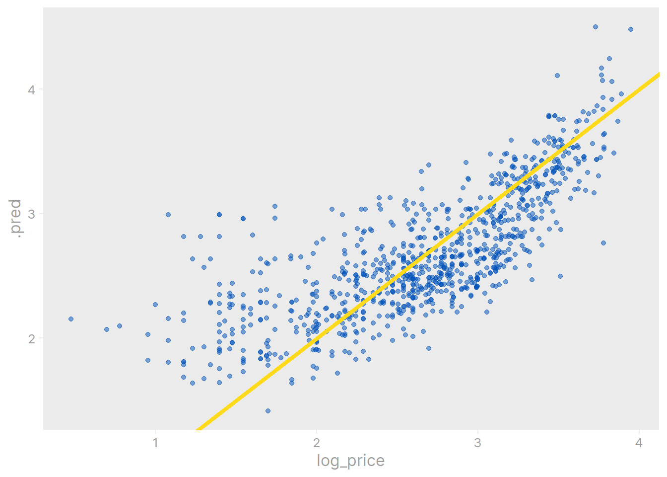

Not as bad as I was expecting, but we can definitely improve on this:

Random forest

Following along with Julia Silge’s approach, I will attempt to tune a random forest model via ranger:

ranger_spec <- rand_forest(mtry = tune(), min_n = tune(), trees = 1000) %>%
  set_mode("regression") %>%
  set_engine("ranger")

ranger_workflow <- workflow() %>%
  add_recipe(ikea_rec) %>%
  add_model(ranger_spec)

# Speed up the tuning with parallel processing
n_cores <- parallel::detectCores(logical = FALSE)
library(doParallel)
cl <- makePSOCKcluster(n_cores - 1)
registerDoParallel(cl)

set.seed(12)

library(tictoc) # A convenient package for timing
tic()
ranger_tune <-
  tune_grid(ranger_workflow, resamples = ikea_bootstrap, grid = 11,
            # This argument is required when running in parallel
            control = control_grid(pkgs = c("textrecipes")))
toc()

226.84 sec elapsed

The 5 best fits to the training data by RMSE:

show_best(ranger_tune, metric = "rmse")

# A tibble: 5 × 8
   mtry min_n .metric .estimator  mean     n std_err .config              
  <int> <int> <chr>   <chr>      <dbl> <int>   <dbl> <chr>                
1    22     3 rmse    standard   0.305    25 0.00225 Preprocessor1_Model08
2     6     8 rmse    standard   0.309    25 0.00205 Preprocessor1_Model11
3    19    15 rmse    standard   0.309    25 0.00210 Preprocessor1_Model09
4    12    18 rmse    standard   0.310    25 0.00212 Preprocessor1_Model01
5    15    20 rmse    standard   0.311    25 0.00211 Preprocessor1_Model07

As expected, we get better performance with the more flexible random forest models compared to linear regression. Choose the best model from the tuning by RMSE:

ranger_best <- ranger_workflow %>%
  finalize_workflow(select_best(ranger_tune, metric = "rmse"))
ranger_best

══ Workflow ════════════════════════════════════════════════════════════════════
Preprocessor: Recipe
Model: rand_forest()

── Preprocessor ────────────────────────────────────────────────────────────────
6 Recipe Steps

• step_impute_mode()
• step_other()
• step_impute_knn()
• step_clean_levels()
• step_dummy()
• step_zv()

── Model ───────────────────────────────────────────────────────────────────────
Random Forest Model Specification (regression)

Main Arguments:
  mtry = 22
  trees = 1000
  min_n = 3

Computational engine: ranger 

The last step is the last_fit() to the training data and evaluating on testing data:

ranger_fit <- last_fit(ranger_best, ikea_split)

The metrics and predictions to the testing data:

collect_metrics(ranger_fit)

# A tibble: 2 × 4
  .metric .estimator .estimate .config             
  <chr>   <chr>          <dbl> <chr>               
1 rmse    standard       0.263 Preprocessor1_Model1
2 rsq     standard       0.833 Preprocessor1_Model1

collect_predictions(ranger_fit) %>%
  ggplot(aes(log_price, .pred)) +
  geom_point(color = ikea_colors[1], alpha = 0.5) +
  geom_abline(color = ikea_colors[2], size = 1.5)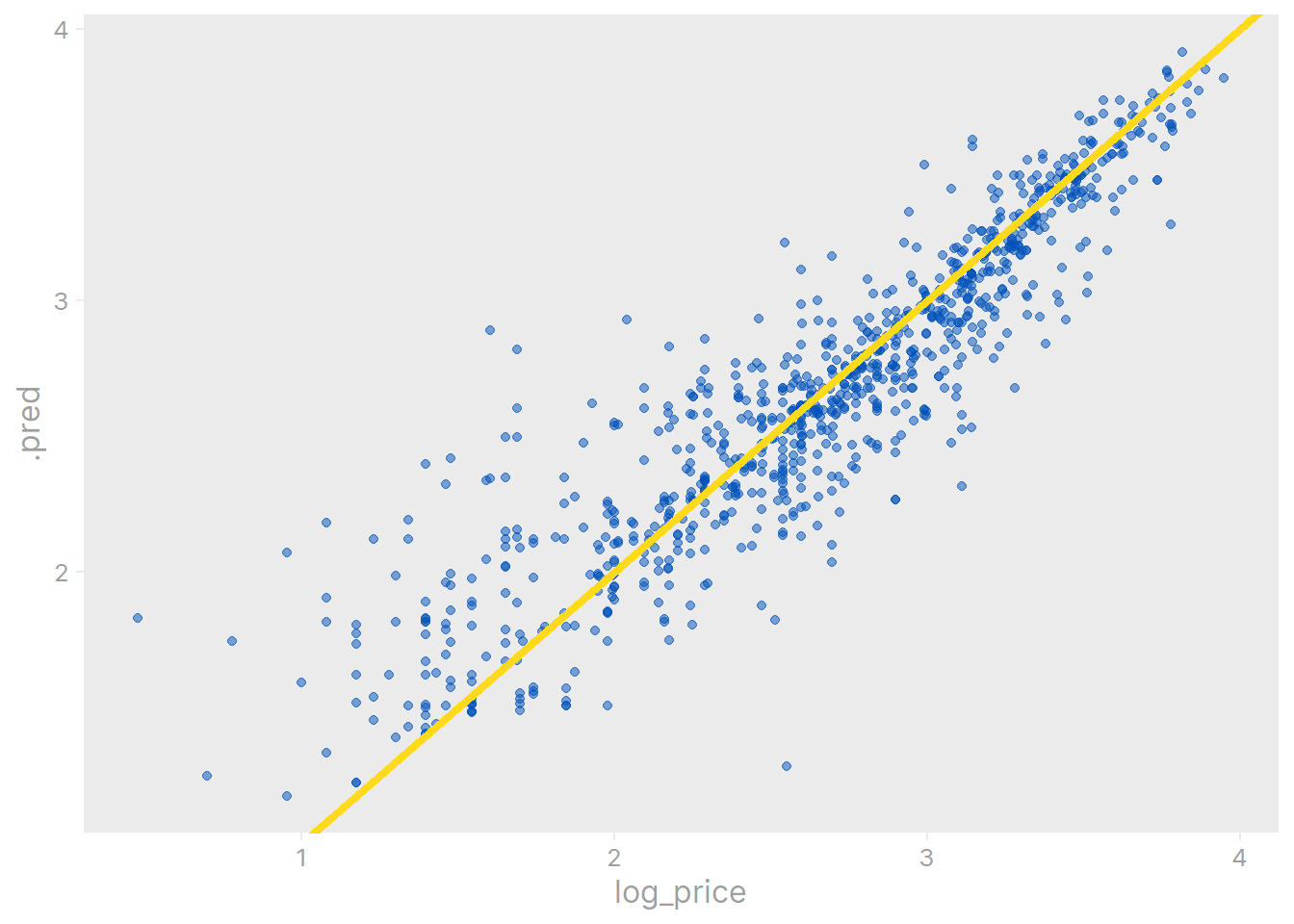

As an example of applying this model, here is a random item:

set.seed(293)
ikea_sample <- ikea %>% slice_sample(n = 1)

ikea_sample %>% glimpse()

Rows: 1
Columns: 25
$ row_number            <dbl> 180
$ item_id               <dbl> 19129932
$ name                  <fct> BRIMNES
$ category              <fct> "Beds"
$ price                 <dbl> 1795
$ old_price             <dbl> NA
$ sellable_online       <lgl> TRUE
$ link                  <fct> https://www.ikea.com/sa/en/p/brimnes-day-bed-w-2…
$ other_colors          <lgl> TRUE
$ short_description     <fct> "Day-bed w 2 drawers/2 mattresses"
$ designer              <fct> "IKEA of Sweden/K Hagberg/M Hagberg"
$ depth                 <dbl> 53
$ height                <dbl> 21
$ width                 <dbl> 86
$ perc_discount         <dbl> 0
$ short_description_dim <fct> 80x200 cm
$ chairs                <dbl> 0
$ stools                <dbl> 0
$ tables                <int> 0
$ sofa_seats            <dbl> 0
$ sofa_bed              <lgl> FALSE
$ sofa_sectional        <lgl> FALSE
$ sofa_type             <fct> Not a sofa
$ designer_group        <fct> IKEA + individual(s)
$ log_price             <dbl> 3.254064

The true price (on the log scale) is 3.25. Our model predicts:

predict(ranger_fit$.workflow[[1]], ikea_sample)

# A tibble: 1 × 1
  .pred
  <dbl>
1  3.16

Which is pretty close.

Lastly, I am interested to see the variable importance of this model, particularly for the engineered features:

library(vip)

# Overwrite the previous random forest specification
ranger_spec_imp <- ranger_spec %>%
  # Specify the best tuning parameters
  finalize_model(select_best(ranger_tune, metric = "rmse")) %>%
  # Alter the engine arguments to compute variable importance
  set_engine("ranger", importance = "permutation")

ranger_fit_imp <- workflow() %>%
  add_recipe(ikea_rec) %>%
  add_model(ranger_spec_imp) %>%
  fit(ikea_train) %>%
  extract_fit_parsnip()

vip(ranger_fit_imp, num_features = 20,
    aesthetics = list(fill = ikea_colors[1])) +
  scale_y_continuous(expand = c(0, 0)) +
  theme(axis.text.y = element_text(face = "bold"))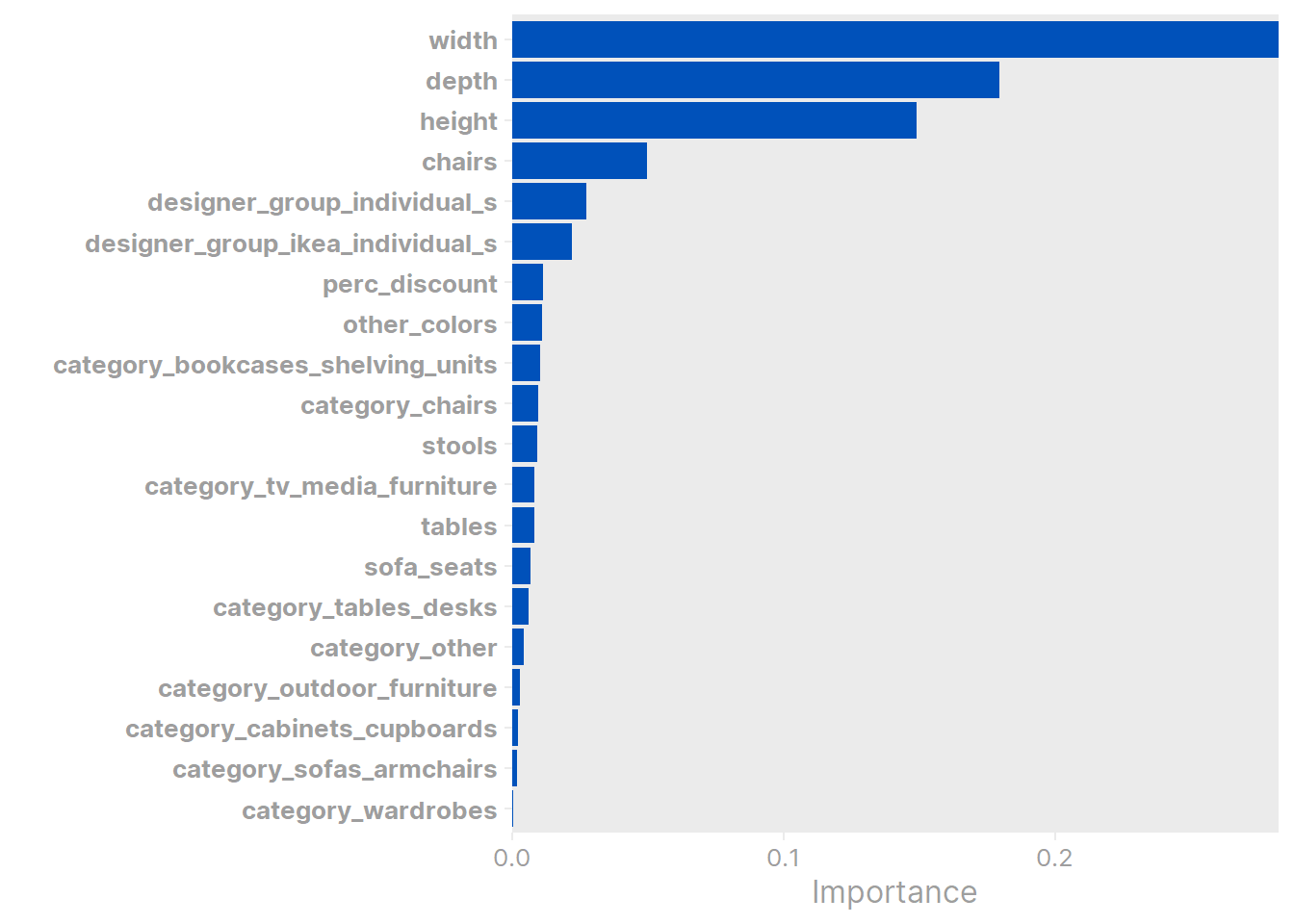

As with Julie Silge’s model, the width/depth/height variables are the most important predictors. The chairs feature, which took some fancy regex to engineer, turned out to be worthwhile as it was the 4th most important predictor here. designer_group ended up being more important than category.

Reproducibility

Session info

 setting  value
 version  R version 4.2.1 (2022-06-23 ucrt)
 os       Windows 10 x64 (build 19044)
 system   x86_64, mingw32
 ui       RTerm
 language (EN)
 collate  English_Canada.utf8
 ctype    English_Canada.utf8
 tz       America/Curacao
 date     2022-10-27
 pandoc   2.18 @ C:/Program Files/RStudio/bin/quarto/bin/tools/ (via rmarkdown)

Git repository

Local:    main C:/Users/tdunn/Documents/tdunn-quarto
Remote:   main @ origin (https://github.com/taylordunn/tdunn-quarto.git)
Head:     [4eb5bf2] 2022-10-26: Added font import to style sheet

Source code, R environment

References

James, Gareth, Daniela Witten, Trevor Hastie, and Robert Tibshirani. 2013. An introduction to statistical learning. Springer.

Footnotes

1. See ISLR section 2.2.2 (James et al. 2013) on the bias-variance trade-off for an accessible explanation of this idea.

Reuse

Citation

BibTeX citation:

@online{dunn2020,
  author = {Dunn, Taylor},
  title = {TidyTuesday 2020 {Week} 45},
  date = {2020-11-08},
  url = {https://tdunn.ca/posts/2020-11-08-tidytuesday-2020-week-45},
  langid = {en}
}

For attribution, please cite this work as:

Dunn, Taylor. 2020. “TidyTuesday 2020 Week 45.” November 8, 2020. https://tdunn.ca/posts/2020-11-08-tidytuesday-2020-week-45.